Space Shuttle Aufstiegsdaten
Original-Fragen der NASA
A. Enter the data from Table 1 into your graphing calculator. Create a scatterplot of the space shuttle’s altitude in relation to time. Use the regression functions on your calculator to determine which type of function best fits the data (i.e. linear, quadratic, cubic, quartic, exponential, power, etc.).
B. Write the function describing the space shuttle’s altitude. Let h stand for altitude and t stand for time. In writing the equation, you will need to decide what decimal place to round the coefficients to. An alternative to this is to write the coefficients using significant figures. In that case, you will need to decide how many significant figures to use. Explain your reasoning for your decision.
C. Using your graphing calculator and the nDeriv command, set Y the altitude function, to be the first derivative and apply the first derivative test to Y, to determine the relative extrema on the interval [0, 520]. Compare the extrema with the data in table 1. How closely does your function represent the data in table 1? What do the extrema represent about the altitude of the space shuttle?
D. Determine the points of inflection of the altitude function. Keep your function needed to find the points of inflection (Wendepunkt) in Y.
E. Analyze the altitude function along the interval [0,160]. What is happening to the space shuttle when the concavity changes?
F. Use your graphing calculator to make a scatterplot of the velocity versus time from Table 1. Explain what is happening to the velocity of the space shuttle over the interval [0, 520]. Is there one function that best fits the data? Why or why not? Be careful to select the correct lists when finding the regressions. What is your velocity function? Let v stand for velocity and t stand for time. Keep this equation in Y
G. Create a scatterplot of acceleration vs. time. What happens to the space shuttle’s acceleration between [0, 100]? Why does the space shuttle’s acceleration increase in a quadratic fashion along the interval [120, 460]? What is happening to the acceleration on the interval [480, 500] and why? Why does the acceleration drop drastically along the interval [500, 520]? What happens to the space shuttle during these time intervals?
H. Is there one regression function that best fits the acceleration data? Why or why not? What is the acceleration function that describes the interval [120, 460]? Let a stand for acceleration and t stand for time. Express the coefficients as three significant figures.
I.Compare the graphs in Y (the first derivative of the altitude function) and in Y (the velocity function found by doing the regression of the data). Do this by turning all other equations off. Do not clear the other equations. Remember to adjust your viewing window. How do these graphs compare? Explain the differences in what they are representing.
J. Now compare the graphs in Y (the second derivative of the altitude function) and in Y (the acceleration function found by doing the regression of the data). How do these graphs compare? Explain the differences in what they are representing.
Quelle
www,nasa,gov/pdf/466711main_AP_ST_ShuttleAscent,pdf
